Risk Prediction
Advanced Statistics for Records Research
Albert Henry
UCL Institute of Health Informatics
Online slides (CC licence: BY-SA-NC):
https://ihi-risk-teaching.netlify.app/
Learning objectives
This lecture will cover:
- Types of prediction
- 2x2 contingency table
- Metrics to evaluate model performance
- Model development and validation
in the context of binary risk prediction
Acknowledgements
Materials and data presented are based on previous slides prepared by L. Palla, D. Prieto, and E. Williamson
Scenario
Consider a dataset consisting some variables collected from a group of individuals. We want to predict which individuals develop a certain binary outcome Y.
Examples
| Population | Available data | Outcome to predict |
|---|---|---|
| Surgical patients | age, sex, comorbidities, medications, severity of disease | complications after surgery |
| Covid-19 patients | age, sex, vaccination status, virus variant, chest X-ray | ICU admission within 10 days |
| Healthy individuals | body mass index, lifestyle, socioeconomic status, genotypes, lipid profile | myocardial infarction in 10-year follow-up |
*Note: prediction modelling is not limited to biomedical problems
Types of prediction: deterministic vs probabilistic
Deterministic:
- Classify each individual into one of the two possible outcomes.
- Often used in (Supervised) Machine Learning
Probabilistic:
- Assign each individual a probability of developing the outcome.
- Often used in Biostatistics and is known as Risk Prediction*
Both methods use individual-level data on a set of variables (or predictors) to develop a prediction model
*Other names: risk prediction model, predictive model, prognostic (or prediction) index or rule, and risk score
Types of prediction: diagnostic vs prognostic

Moons KGM, Altman DG, Reitsma JB, et al. Ann Intern Med. 2015 Jan 6;162(1):W1–73.
Example
Who will develop myocardial infarction in the next 5 years?
| id | age | sex | diabet | SBP | Classify | Predict | Observed |
|---|---|---|---|---|---|---|---|
| 1 | 35 | F | Yes | 145 | |||
| 2 | 35 | M | No | 130 | |||
| 3 | 55 | F | No | 115 | |||
| 4 | 55 | M | Yes | 170 | |||
| 5 | 65 | F | No | 135 | |||
| 6 | 65 | M | Yes | 140 | |||
| 7 | 75 | M | Yes | 160 | |||
| 8 | 75 | F | No | 130 | |||
| 9 | 85 | F | Yes | 130 | |||
| 10 | 85 | M | No | 160 |
Deterministic classification
Suppose we have a pre-defined deterministic classification model C:
C(age, sex, diabet, SBP) = 0 or 1
| id | age | sex | diabet | SBP | Classify | Predict | Observed |
|---|---|---|---|---|---|---|---|
| 1 | 35 | F | Yes | 145 | No | ||
| 2 | 35 | M | No | 130 | No | ||
| 3 | 55 | F | No | 115 | No | ||
| 4 | 55 | M | Yes | 170 | Yes | ||
| 5 | 65 | F | No | 135 | No | ||
| 6 | 65 | M | Yes | 140 | Yes | ||
| 7 | 75 | M | Yes | 160 | Yes | ||
| 8 | 75 | F | No | 130 | No | ||
| 9 | 85 | F | Yes | 130 | Yes | ||
| 10 | 85 | M | No | 160 | Yes |
Probabilistic prediction
Suppose we have a pre-defined probabilistic prediction model P:
P(age, sex, diabet, SBP) = [0, 1]
| id | age | sex | diabet | SBP | Classify | Predict | Observed |
|---|---|---|---|---|---|---|---|
| 1 | 35 | F | Yes | 145 | No | 0.15 | |
| 2 | 35 | M | No | 130 | No | 0.05 | |
| 3 | 55 | F | No | 115 | No | 0.10 | |
| 4 | 55 | M | Yes | 170 | Yes | 0.55 | |
| 5 | 65 | F | No | 135 | No | 0.30 | |
| 6 | 65 | M | Yes | 140 | Yes | 0.52 | |
| 7 | 75 | M | Yes | 160 | Yes | 0.60 | |
| 8 | 75 | F | No | 130 | No | 0.40 | |
| 9 | 85 | F | Yes | 130 | Yes | 0.55 | |
| 10 | 85 | M | No | 160 | Yes | 0.60 |
Observation
... after 5 years follow-up
| id | age | sex | diabet | SBP | Classify | Predict | Observed |
|---|---|---|---|---|---|---|---|
| 1 | 35 | F | Yes | 145 | No | 0.15 | No |
| 2 | 35 | M | No | 130 | No | 0.05 | No |
| 3 | 55 | F | No | 115 | No | 0.10 | No |
| 4 | 55 | M | Yes | 170 | Yes | 0.55 | No |
| 5 | 65 | F | No | 135 | No | 0.30 | Yes |
| 6 | 65 | M | Yes | 140 | Yes | 0.52 | No |
| 7 | 75 | M | Yes | 160 | Yes | 0.60 | Yes |
| 8 | 75 | F | No | 130 | No | 0.40 | No |
| 9 | 85 | F | Yes | 130 | Yes | 0.55 | Yes |
| 10 | 85 | M | No | 160 | Yes | 0.60 | Yes |
Model validation
Both
CandPmodels are not always correct in predicting the outcomeThe goal of model validation is to evaluate model performance by comparing predictions against observed values.
For binary prediction, model validation usually starts with creating a 2x2 contingency table / confusion matrix consisting all four possible pairs of predicted-observed values
2x2 contingency table / Confusion matrix
| id | Predicted | Observed |
|---|---|---|
| 1 | No | No |
| 2 | No | No |
| 3 | No | No |
| 4 | Yes | No |
| 5 | No | Yes |
| 6 | Yes | No |
| 7 | Yes | Yes |
| 8 | No | No |
| 9 | Yes | Yes |
| 10 | Yes | Yes |
2x2 contingency table / Confusion matrix
| id | Predicted | Observed |
|---|---|---|
| 1 | No | No |
| 2 | No | No |
| 3 | No | No |
| 4 | Yes | No |
| 5 | No | Yes |
| 6 | Yes | No |
| 7 | Yes | Yes |
| 8 | No | No |
| 9 | Yes | Yes |
| 10 | Yes | Yes |
| Predicted | Observed | Count |
|---|---|---|
| Yes | Yes | 3 |
| Yes | No | 2 |
| No | Yes | 1 |
| No | No | 4 |
| Predicted | Observed | Term |
|---|---|---|
| + | + | True Positive |
| + | - | False Positive |
| - | + | False Negative |
| - | - | True Negative |
2x2 contingency table / Confusion matrix
Observed |
||
|---|---|---|
| Predicted | + | - |
| + | 3 | 2 |
| - | 1 | 4 |
Observed |
||
|---|---|---|
| Predicted | + | - |
| + | True Positive | False Positive |
| - | False Negative | True Negative |
With 2 x 2 contingency table, we can calculate several useful metrics* to evaluate model performance, including:
sensitivity, recall, hit / detection rate, or true positive rate (TPR)
specificity, selectivity, or true negative rate (TNR)
precision or positive predictive value (PPV)
negative predictive value (NPV)
*for a full list, refer to Wikipedia entry for Confusion matrix
Sensitivity
a.k.a True Positive Rate, Recall, Hit / Detection Rate
Probability of correctly predicting positive outcome
What is the probability of a positive classification, given a positive outcome?
P(^Y=1 | Y=1)
Observed |
||
|---|---|---|
| Predicted | + | - |
| + | TP | FP |
| - | FN | TN |
Sensitivity=∑True Positive∑Observed Positive Sensitivity=TPTP+FN
Specificity
a.k.a Selectivity, True Negative Rate
Probability of correctly predicting ngative outcome
What is the probability of a negative classification, given a negative outcome?
P(^Y=0 | Y=0)
Observed |
||
|---|---|---|
| Predicted | + | - |
| + | TP | FP |
| - | FN | TN |
Specificity=∑True Negative∑Observed Negative Specificity=TNTN+FP
Positive predictive value (PPV)
Probability of a positive outcome given a positive classification
P(Y=1 | ^Y=1)
For a given model (e.g. diagnostic test) with fixed sensitivity and specificity, PPV is positively correlated with disease prevalence
Intuition: as prevalence increases, true positive increases while false positives decreases
Observed |
||
|---|---|---|
| Predicted | + | - |
| + | TP | FP |
| - | FN | TN |
PPV=∑True Positive∑Predicted Positive PPV=TPTP+FP
Negative predictive value (NPV)
Probability of a negative outcome given a negative classification
P(Y=0 | ^Y=0)
For a given model (e.g. diagnostic test) with fixed sensitivity and specificity, NPV is negatively correlated with disease prevalence
Intuition: as prevalence increases, true negative decreases while false negative increases
Observed |
||
|---|---|---|
| Predicted | + | - |
| + | TP | FP |
| - | FN | TN |
NPV=∑True Negative∑Predicted Negative NPV=TNTN+FN
Comparing classifications with observations
Suppose we have the following contingency table for classification model C:
Observed |
|||
|---|---|---|---|
| Predicted | + | - | Total |
| + | 3 | 2 | 5 |
| - | 1 | 4 | 5 |
| Total | 4 | 6 | 10 |
Sensitivity = ?
Specificity = ?
PPV = ?
NPV = ?
Comparing classifications with observations
Suppose we have the following contingency table for classification model C:
Observed |
|||
|---|---|---|---|
| Predicted | + | - | Total |
| + | 3 | 2 | 5 |
| - | 1 | 4 | 5 |
| Total | 4 | 6 | 10 |
Sensitivity = 3/4 = 0.75
Specificity = 4/6 = 0.67
PPV = 3/5 = 0.6
NPV = 4/5 = 0.8
Comparing predictions with observations
For prediction model P, we order by predicted probability and choose a cut-off point to classify as "Yes", e.g.
"Yes" if probability (P) > 0.1
| id | Predict | Observed | Prob >0.1 |
|---|---|---|---|
| 2 | 0.05 | No | No |
| 3 | 0.10 | No | No |
| 1 | 0.15 | No | Yes |
| 5 | 0.30 | Yes | Yes |
| 8 | 0.40 | No | Yes |
| 6 | 0.52 | No | Yes |
| 4 | 0.55 | No | Yes |
| 9 | 0.55 | Yes | Yes |
| 7 | 0.60 | Yes | Yes |
| 10 | 0.60 | Yes | Yes |
Cut-off point: Yes if P > 0.1
Observed |
|||
|---|---|---|---|
| Predicted | + | - | Total |
| + | 4 | 4 | 8 |
| - | 0 | 2 | 2 |
| Total | 4 | 6 | 10 |
Sensitivity = 4/4 = 1
Specificity = 2/6 = 0.33
PPV = 4/8 = 0.5
NPV = 2/2 = 1
Higher sensitivity, lower specificity than classification model C
Cut-off point: Yes if P > 0.4
| id | Predict | Observed | Prob >0.4 |
|---|---|---|---|
| 2 | 0.05 | No | No |
| 3 | 0.10 | No | No |
| 1 | 0.15 | No | No |
| 5 | 0.30 | Yes | No |
| 8 | 0.40 | No | No |
| 6 | 0.52 | No | Yes |
| 4 | 0.55 | No | Yes |
| 9 | 0.55 | Yes | Yes |
| 7 | 0.60 | Yes | Yes |
| 10 | 0.60 | Yes | Yes |
Cut-off point: Yes if P > 0.4
Observed |
|||
|---|---|---|---|
| Predicted | + | - | Total |
| + | 3 | 2 | 5 |
| - | 1 | 4 | 5 |
| Total | 4 | 6 | 10 |
Sensitivity = 3/4 = 0.75
Specificity = 4/6 = 0.67
PPV = 3/5 = 0.6
NPV = 4/5 = 0.8
Same contingency table as classification model C
Cut-off point: Yes if P > 0.55
| id | Predict | Observed | Prob >0.55 |
|---|---|---|---|
| 2 | 0.05 | No | No |
| 3 | 0.10 | No | No |
| 1 | 0.15 | No | No |
| 5 | 0.30 | Yes | No |
| 8 | 0.40 | No | No |
| 6 | 0.52 | No | No |
| 4 | 0.55 | No | No |
| 9 | 0.55 | Yes | No |
| 7 | 0.60 | Yes | Yes |
| 10 | 0.60 | Yes | Yes |
Cut-off point: Yes if P > 0.55
Observed |
|||
|---|---|---|---|
| Predicted | + | - | Total |
| + | 2 | 0 | 2 |
| - | 2 | 6 | 8 |
| Total | 4 | 6 | 10 |
Sensitivity = 2/4 = 0.5
Specificity = 6/6 = 1
PPV = 2/2 = 1
NPV = 6/8 = 0.75
Lower sensitivity, higher specificity than classification model C
All cut-off points
If we repeat this process for each probability value, we can obtain a list of sensitivity and specificity values
| id | Predict | Observed | Cut-off | Sensitivity | Specificity |
|---|---|---|---|---|---|
| 2 | 0.05 | No | P >0.05 | 1.00 | 0.17 |
| 3 | 0.10 | No | P >0.1 | 1.00 | 0.33 |
| 1 | 0.15 | No | P >0.15 | 1.00 | 0.50 |
| 5 | 0.30 | Yes | P >0.3 | 0.75 | 0.50 |
| 8 | 0.40 | No | P >0.4 | 0.75 | 0.67 |
| 6 | 0.52 | No | P >0.52 | 0.75 | 0.83 |
| 4 | 0.55 | No | P >0.55 | 0.50 | 1.00 |
| 9 | 0.55 | Yes | P >0.55 | 0.50 | 1.00 |
| 7 | 0.60 | Yes | P >0.6 | 0.00 | 1.00 |
| 10 | 0.60 | Yes | P >0.6 | 0.00 | 1.00 |
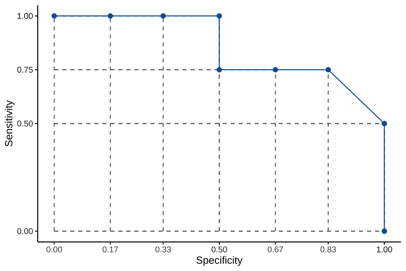
Receiver Operating Characterictic (ROC) Curve
A curve linking all the sensitivity against the specificity values
| Sens | Spec |
|---|---|
| 1.00 | 0.17 |
| 1.00 | 0.33 |
| 1.00 | 0.50 |
| 0.75 | 0.50 |
| 0.75 | 0.67 |
| 0.75 | 0.83 |
| 0.50 | 1.00 |
| 0.50 | 1.00 |
| 0.00 | 1.00 |
| 0.00 | 1.00 |

Area Under the [ROC] Curve (AUC / AUROC)
What is the AUC?
Area Under the [ROC] Curve (AUC / AUROC)
What is the AUC?
Sample calculation with yardstick package in R
# df = the dataset shown in previous slidesroc <- yardstick::roc_auc(df, truth = Observed, Predict)roc## # A tibble: 1 × 3## .metric .estimator .estimate## <chr> <chr> <dbl>## 1 roc_auc binary 0.854AUC = 0.8541667
AUC and the distributions of predictors in the two outcome groups at different cut-off values

by Dariya Sydykova (follow link for more info)

What does AUC tell us?
AUC estimates the probability that a randomly chosen observed “yes” was assigned a higher probability than a randomly observed “no” by the model
Real world models will have AUC from 0.5 to 1. A value closer to 1 indicates better performance in separating "yes" and "no".
For binary classification, AUC is equal to concordance (C) statistic
How do we come up with predictions?
We propose a statistical model for the probability of the event happening P(Yi=1) depending on the other variables
For example a logistic model:
log(P(Yi=1)1−P(Yi=1))=β0+β1Xi+β2Zi+⋯(1)
We need a training set where we can observe all the variables Yi,Xi,Zi,… to estimate the coefficients β0,β1,β2,…
Once we have the coefficients that best fit the data we can calculate the predicted risk for each individual i
ˆP(Yi=1)=eˆβ0+ˆβ1Xi+ˆβ2Zi+⋯1+eˆβ0+^β1Xi+^β2Zi+⋯(2)
Dataset for model development & model validation
Internal validation
The validity of claims for the underlying population where the data originated from (reproducibility)
Split sample validation: split dataset randomly into training (for model development) and test set (for validation)
Other methods: cross validation and bootstrap resampling
External validation
Generalizability of claims to ‘plausibly related’ populations not included in the initial study population (transportability)
e.g. temporal or geographical validation
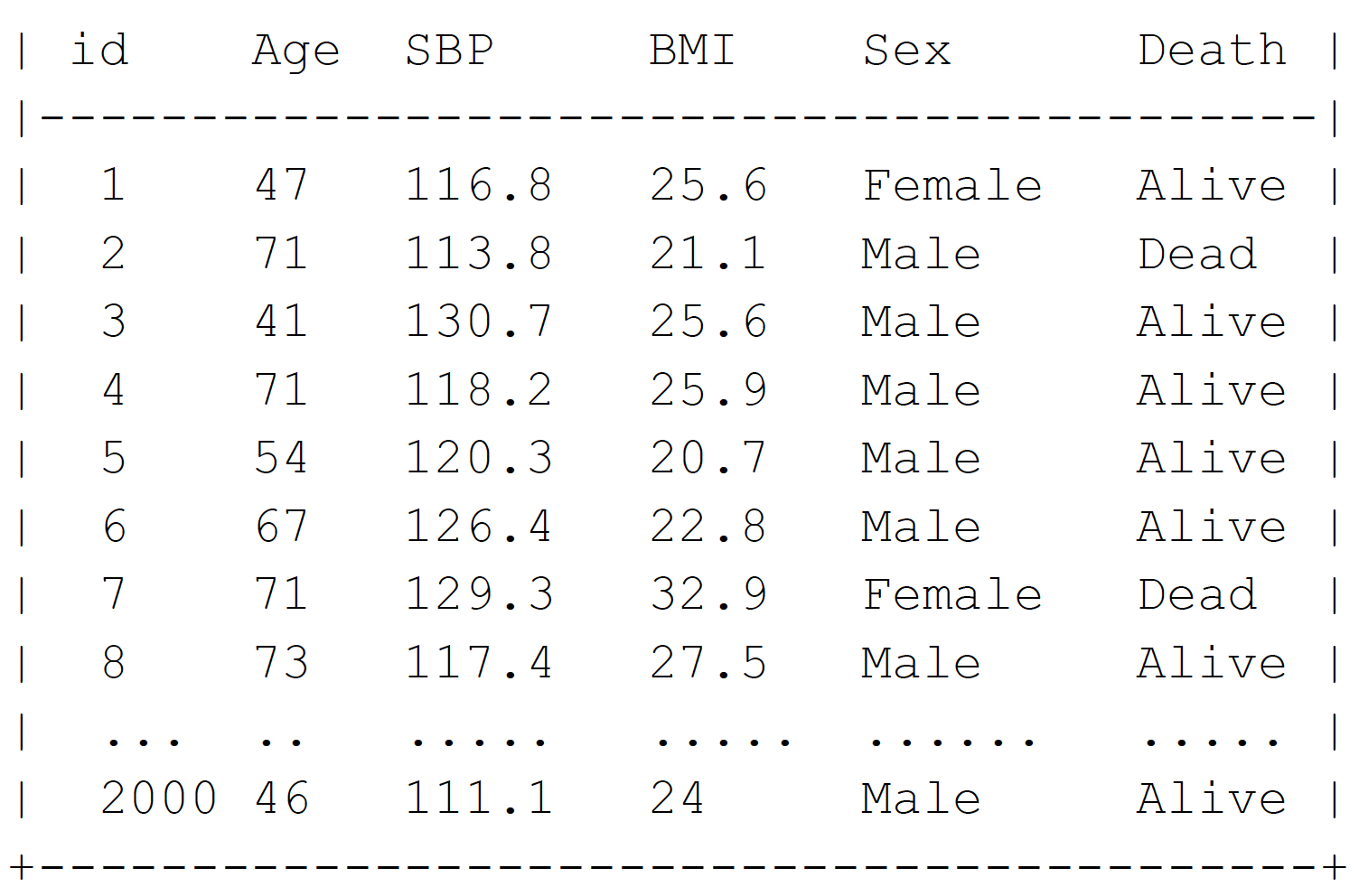
A larger example with 2000 individuals
We will use the variables Age, Sex, SBP, and BMI to predict if the person will be dead (Death = 1) or alive (Death= 0) in 5 years time
Model M1: Logistic regression
Stata command:
logistic dead age sex sbp bmi
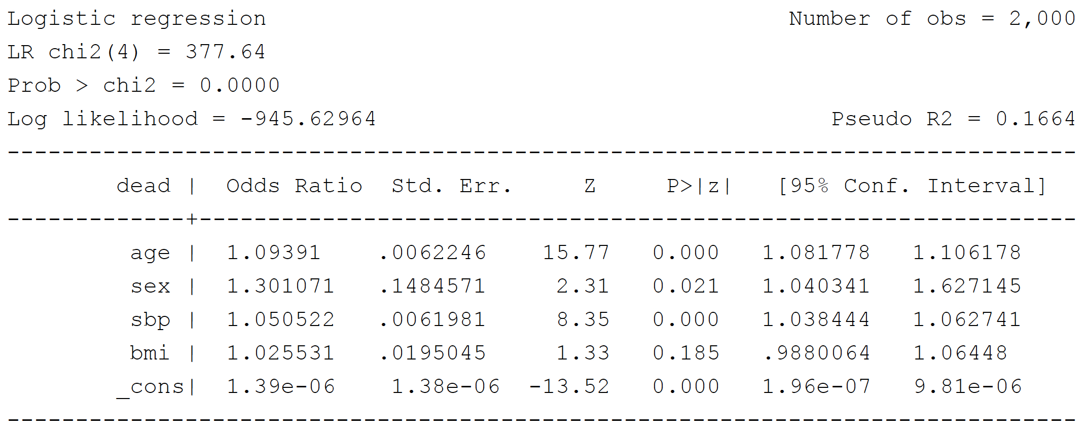
Note that BMI is not statistically significant (P = 0.185)
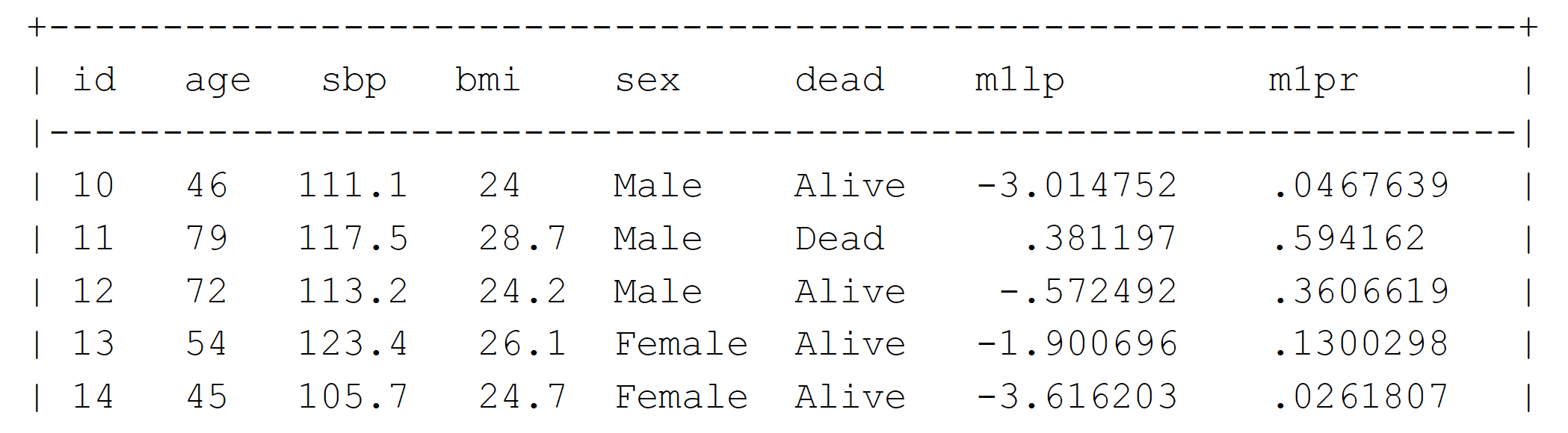
Make predictions from Model M1
Create variable: logit of the probability of death - equation (1)
predict m1lp, xb
Create variable: predicted probability of death - equation (2)
predict m1pr
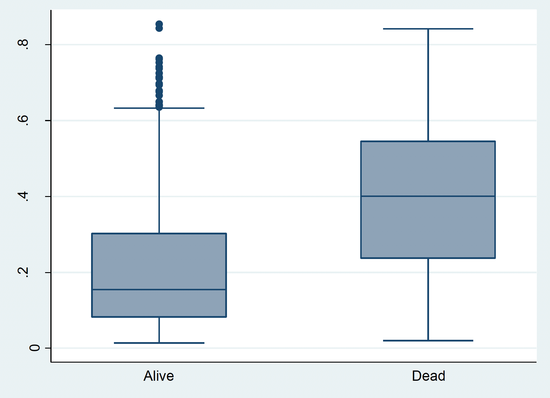
Predicted probability of death in dead and alive group
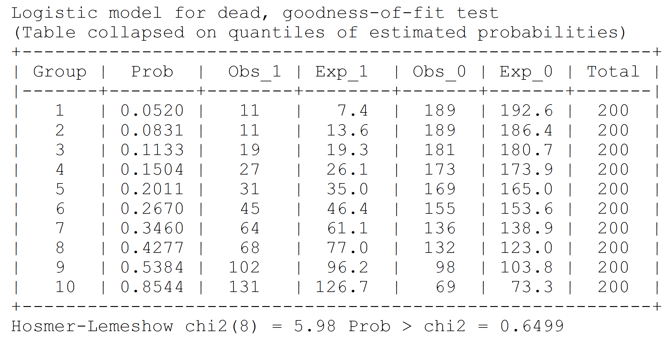
Model calibration
Evaluate goodness of fit with Hosmer-Lemeshow test
estat gof, group(10) table
Model calibration
Goodness of fit: Observed and expected events by deciles of risk
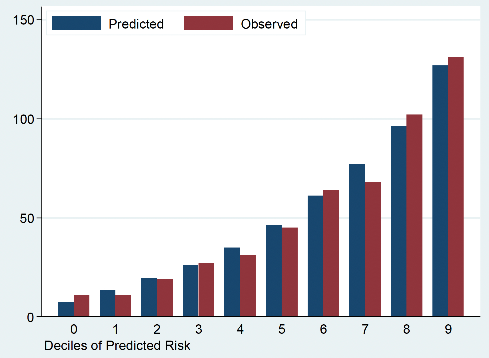
Model calibration
Goodness of fit: Observed and expected events by deciles of risk
Limitation: Hosmer-Lemeshow test can not tell the direction of miscalibration and relies on arbitrary grouping
Model calibration with calibration plot
Calibration-in-the-large: compares average predicted risk with observed risk (0: ideal, <0: underestimation, >0: overestimation)
Calibration slope: evaluate spread of estimated risk (1: ideal, <1: too extreme, >1: too moderate)
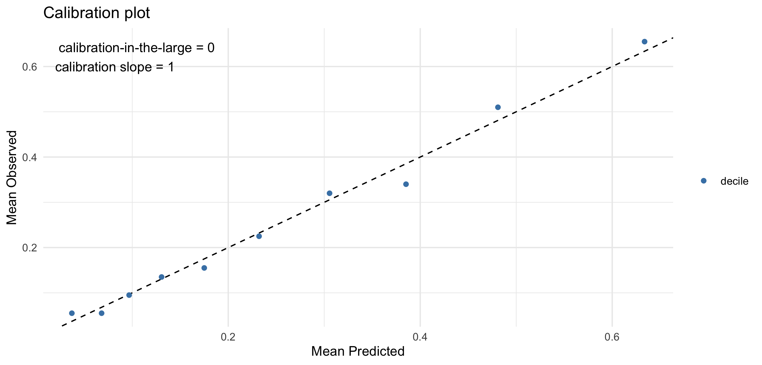
Further discussion: Steyerberg EW, Vergouwe Y (2014) and Calster BV et al. (2019)
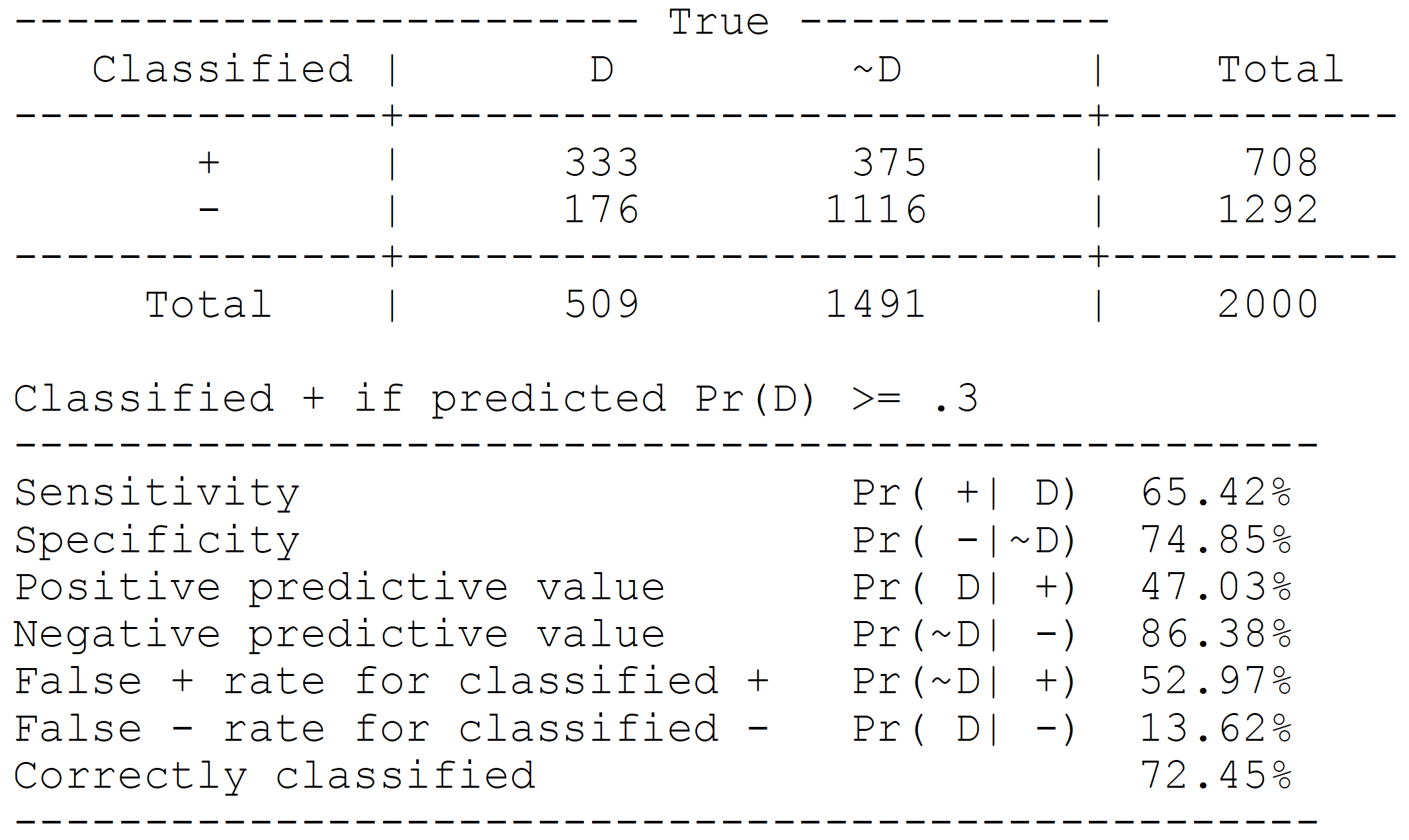
Contingency table: cut-off P(Y=1)≥0.3
estat classification, cutoff(0.3)
ROC curve from model M1
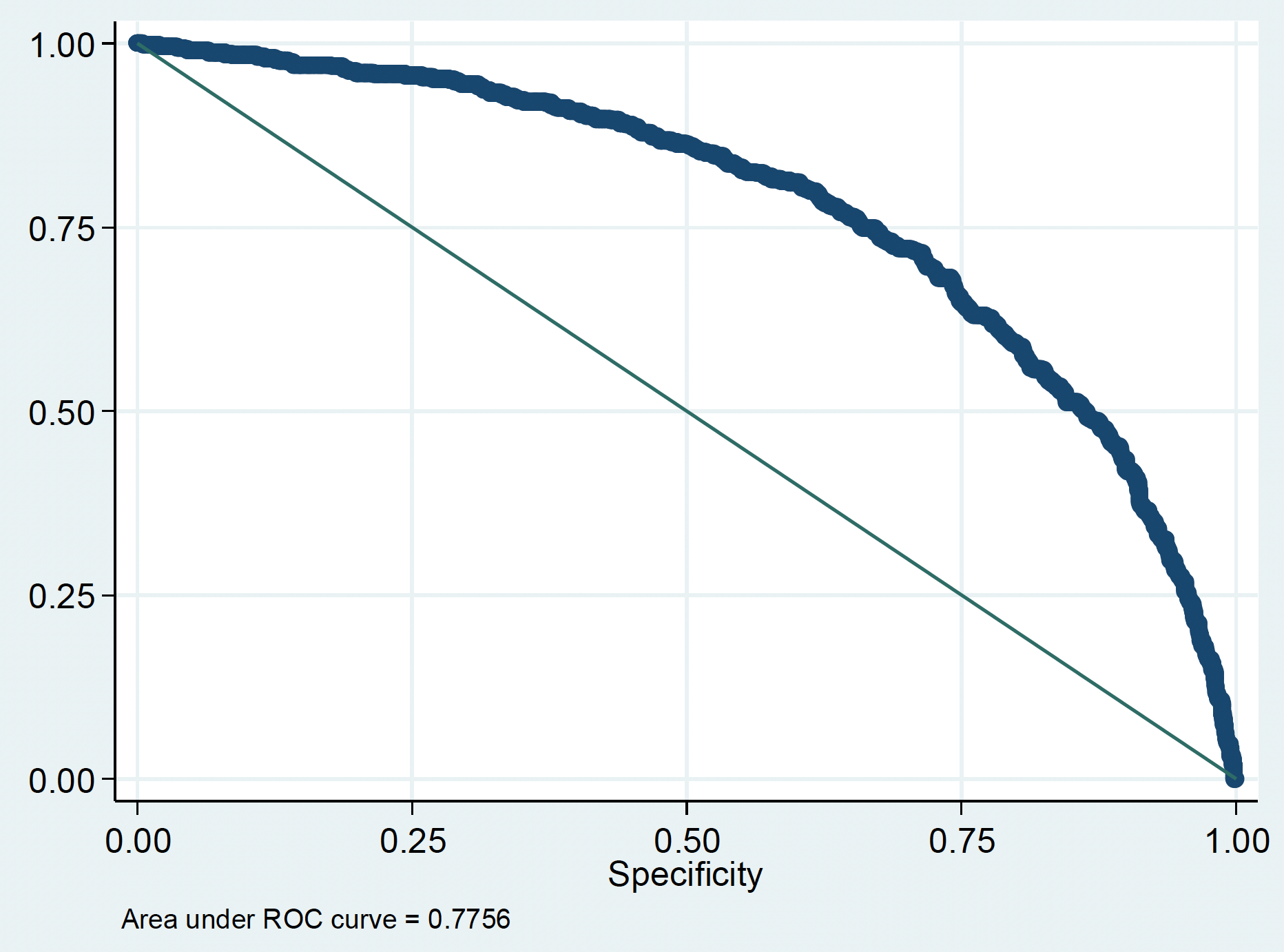
AUC = 0.78
There is a 78% probability that a person who died is assigned a higher predicted risk by the model than a person was alive by the end of the follow up
Sensitivity and Specificity for model M1
by cut-off value
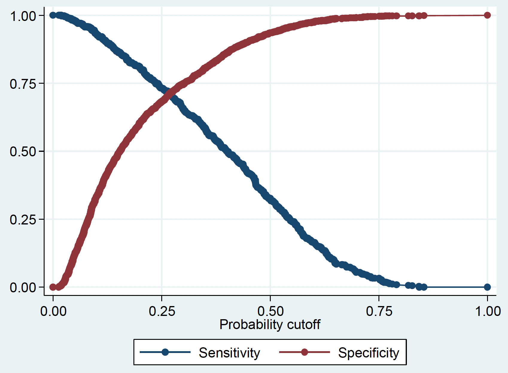
Plotting sensitivity and specificity against cut-off value can help to select the most appropriate cut-off
In practice, this trade-off often needs to be decided on a case-by-case basis
Evaluating prediction model performance
Calibration
- The agreement between the predicted & observed outcomes
- For a group of patients with 10% predicted risk, do 10% experience the outcome?
- e.g. Goodness of fit test, calibration curve
Discrimination
- The ability of the model to distinguish between positive and negative outcome
- e.g. AUC / C statistic
Clinical usefulness
- Does the model provide accurate predictions at the patient level that can be used to guide clinical decision making?
- e.g. Decision curve analysis
Summary
Prediction modelling can be broadly categorised into deterministic and probabilistic methods
2 x 2 contingency table / confusion matrix is useful as a first step to evaluate model performance
AUC is a useful measure of the model discrimination
Comparing observed and predicted risks is useful for model calibration
Assessing clinical usefulness requires other approaches and often requires insights from beyond the data
References and further reading
Practical article: Steyerberg EW, Vergouwe Y. Towards better clinical prediction models: seven steps for development and an ABCD for validation. Eur Heart J. 2014 Aug 1;35(29):1925–1931.
Comparison with machine learning: Breiman L. Statistical Modeling: The Two Cultures (with comments and a rejoinder by the author). Stat Sci. Institute of Mathematical Statistics; 2001 Aug;16(3):199–231.